Under-Damped System (ξ < 1)
Watch videoComments
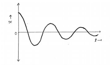 Fig-1
Fig-1
Underdamped system
If the damping factor is less than one or the damping coefficient is less than critical damping coefficient , then the system is said to be an under-damped system.
- We know that roots of differential equations are:
- But for ; the roots for under-damped system are given by and as below:
Where is the imaginary unit of complex root
- The roots are complex and negative, so the solution of differential equation is given by


- According to Euler’s theorem, above equation can be written as:
-
Above equation shows the equation of motion for an underdamped system, and the amplitude reduces gradually and finally becomes zero after some time.
-
Amplitude decreases by
-
The natural angular frequency of damped free vibrations is given by:
- Time period for under-damped vibration is given by:
Suggested Notes:
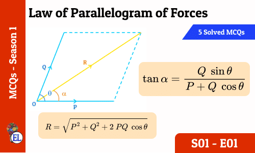
Law of Parallelogram of Forces : 5 in 5 MCQs S01-E01
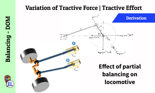
Variation of Tractive Force | Tractive Effort | Effect of Partial Balancing of Locomotives
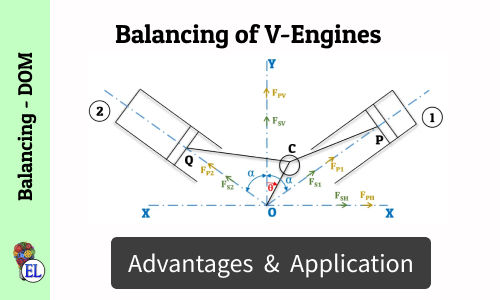
Balancing of V-Engines
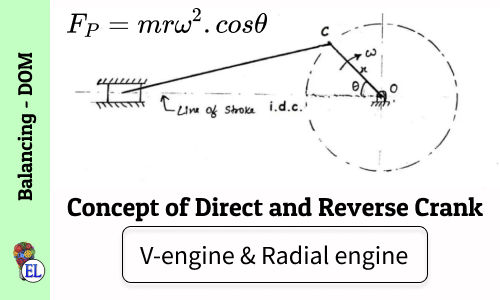
Concept of Direct and Reverse Crank for V-engines & Radial engines
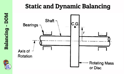
Static and Dynamic Balancing
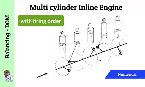
Multi Cylinder Inline Engine (with firing order) | Numerical
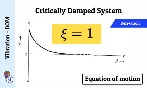
Critically Damped System (ξ = 1)
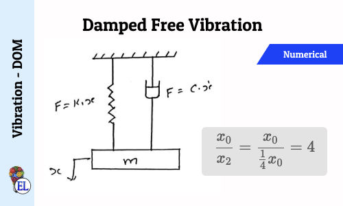
Damped free Vibration - Numerical 1
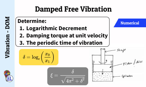
Damped free Vibration - Numerical 2
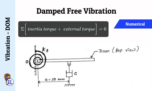
Damped free Vibration - Numerical 4
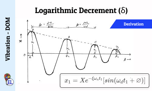
Logarithmic Decrement (δ)
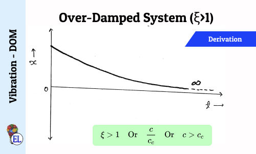
Over-Damped System (ξ>1)
Suggested Notes:
Law of Parallelogram of Forces : 5 in 5 MCQs S01-E01
Variation of Tractive Force | Tractive Effort | Effect of Partial Balancing of Locomotives
Balancing of V-Engines
Concept of Direct and Reverse Crank for V-engines & Radial engines
Static and Dynamic Balancing
Multi Cylinder Inline Engine (with firing order) | Numerical
Critically Damped System (ξ = 1)
Damped free Vibration - Numerical 1
Damped free Vibration - Numerical 2
Damped free Vibration - Numerical 4
Logarithmic Decrement (δ)
Over-Damped System (ξ>1)
Comments:
All comments that you add will await moderation. We'll publish all comments that are topic related, and adhere to our Code of Conduct.
Want to tell us something privately? Contact Us
Post comment