Modified Distribution Method (MODI) | Transportation Problem | Transportation Model
Watch videoTo understand the methods which will be helpful to optimize your solution to transportation problems, we must have the knowledge of optimality tests first.
Jump to Modified Distribution Method (MODI) or Stepping Stone Method for optimizing solution to transportation problem.
Optimality Test:
→ Optimality test is carried to check whether the basic feasible solution (BFS) obtained by any of different methods ( Vogel's Approximation Method (VAM), Least Cost Method or North West Corner Method | Method to Solve Transportation Problem | Transportation Model ) is optimum or not!
→ This test is done only after fulfilling two requirements as follows:
a) Total number of non-negative allocation is (m+n-1).
b) These allocations are in independent cells.where,
m = no. of rows &
n = no. of columns
→ There are two different methods used for checking whether the solution to transportation problem is optimal or not.
Why we should use MODI method ?
→ In Stepping stone method there are 'm' rows and 'n' columns, so the total number of unoccupied cell will be equal to .
→ Thus, total number of loops increases, which increases calculation and it will be more time consuming.
→ Moreover in MODI method, cell evaluations of all the unoccupied cells are calculated simultaneously and only one closed path for the most negative cell is traced.
→ Thus, it saves time over Stepping stone method.
MODI method is also known as "u-v Method".
Let us now understand how Modified Distribution Method (MODI) works. We will understand it using a numerical as follows:
Applying Modified Distribution Method (MODI) - Numerical
Question : Check optimality of the basic feasible solution given below by using MODI method.
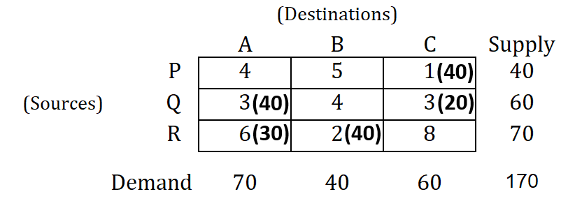 Fig-1: Question
Solution :
Note that all the explanation is provided in “CYAN” colour. You have to write in examination the only thing which are given in this regular colour under each steps (if any), else you can directly solve matrix of the problem as explained here.
→ Prepare a cost matrix by writing cost in allocated cells.
→ Now, introduce dual variables (u & v) corresponding to supply and demand constraints.
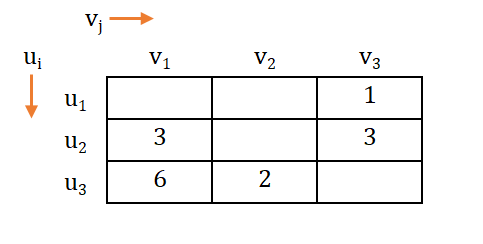 Fig-2: Introducing dual variables
Note that, here dual variables ui and vj are such that, ui + vj = cij (where & ).
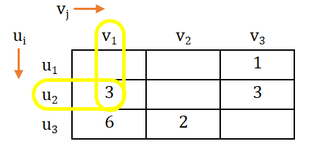 Fig-3: Equations using dual variables
→ As per the note above, we can derive equation as follows:


→ Now, we take either of the variable as '0'.
→ Let, u3 = 0, and then calculating the value of other dual variable, we get;
→ Replacing the values of dual variables in the matrix, we get;
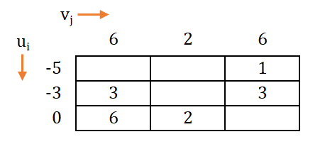 Fig-4: Plotting values of dual variables
→ Now, let us carry out Vacant Cell Evaluation.
→ Vacant cell evaluation is carried out by taking difference for each unoccupied call.
Remember that is known as Implicit cost.
Implicit cost: It is the summation of dual variables of row and columns for each unoccupied cell.
→ Vacant cells are to be filled using above formula as follows:
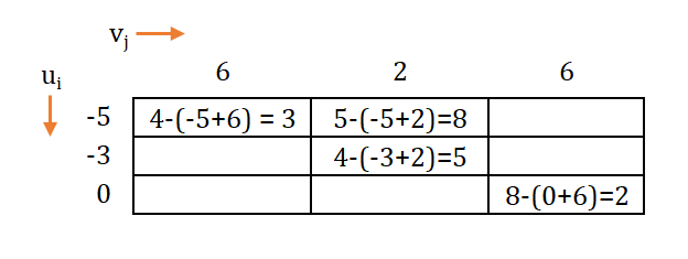 Fig-5: Vacant cell evaluation
Notes :
In this method after performing vacant cell evaluation, if the values of the cells are/is :
(i) Positive (+) → then the current basic feasible solution (BFS) is optimal and stop the procedure. If we alter the present solution, the solution will become poorer.
(ii) Zero (0) → then also the current basic feasible solution (BFS) is optimal, but alternate allocation are possible with same transportation cost.
(iii) Negative (-) → then the obtained solution is not optimal and further improvement is possible.
→ As all the values in the non-allocated cells are now obtained positive (+) by using vacant cell evaluation, the present solution is optimal.
You can find out solution to this numerical through Stepping Stone Method as well.
Suggested Notes:
Stepping Stone | Transportation Problem | Transportation Model
Vogel’s Approximation Method (VAM) | Method to Solve Transportation Problem | Transportation Model
Transportation Model - Introduction
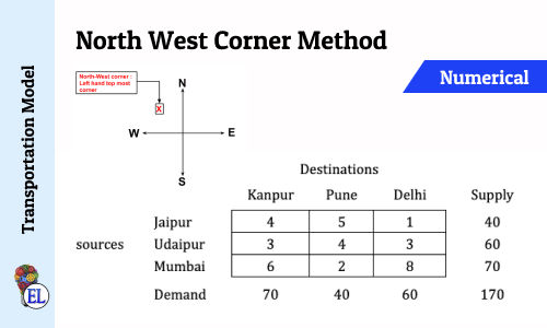
North West Corner Method | Method to Solve Transportation Problem | Transportation Model
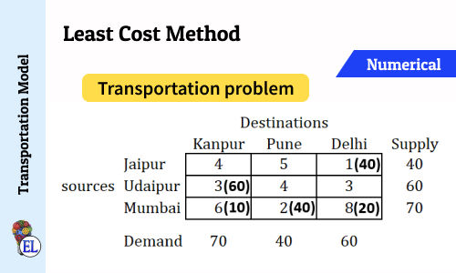
Least Cost Method | Method to Solve Transportation Problem | Transportation Model
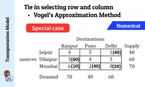
Tie in selecting row and column (Vogel's Approximation Method - VAM) | Numerical | Solving Transportation Problem | Transportation Model
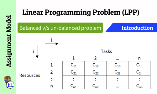
Assignment Model | Linear Programming Problem (LPP) | Introduction
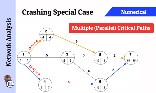
Crashing Special Case - Multiple (Parallel) Critical Paths
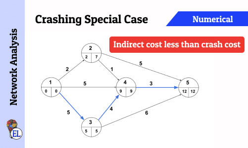
Crashing Special Case - Indirect cost less than Crash Cost
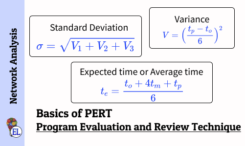
Basics of Program Evaluation and Review Technique (PERT)
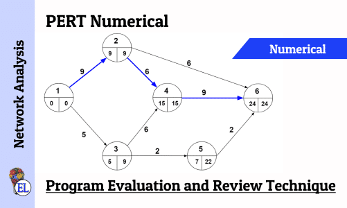
Numerical on PERT (Program Evaluation and Review Technique)
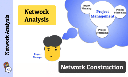
Network Analysis - Dealing with Network Construction Basics
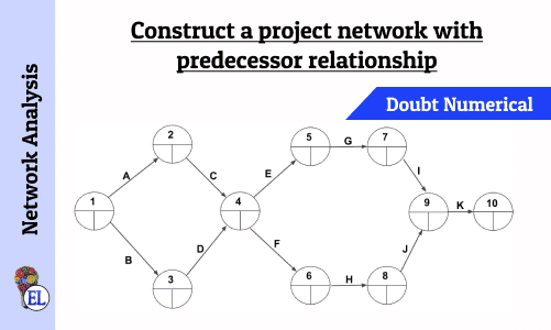
Construct a project network with predecessor relationship | Operation Research | Numerical
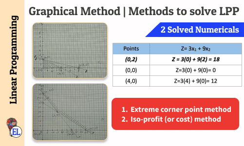
Graphical Method | Methods to solve LPP | Linear Programming
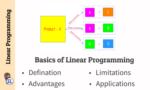
Basics of Linear Programming
Linear Programming Problem (LPP) Formulation with Numericals
Suggested Notes:
Stepping Stone | Transportation Problem | Transportation Model
Vogel’s Approximation Method (VAM) | Method to Solve Transportation Problem | Transportation Model
Transportation Model - Introduction
North West Corner Method | Method to Solve Transportation Problem | Transportation Model
Least Cost Method | Method to Solve Transportation Problem | Transportation Model
Tie in selecting row and column (Vogel's Approximation Method - VAM) | Numerical | Solving Transportation Problem | Transportation Model
Assignment Model | Linear Programming Problem (LPP) | Introduction
Crashing Special Case - Multiple (Parallel) Critical Paths
Crashing Special Case - Indirect cost less than Crash Cost
Basics of Program Evaluation and Review Technique (PERT)
Numerical on PERT (Program Evaluation and Review Technique)
Network Analysis - Dealing with Network Construction Basics
Construct a project network with predecessor relationship | Operation Research | Numerical
Graphical Method | Methods to solve LPP | Linear Programming
Basics of Linear Programming
Linear Programming Problem (LPP) Formulation with Numericals
Comments:
All comments that you add will await moderation. We'll publish all comments that are topic related, and adhere to our Code of Conduct.
Want to tell us something privately? Contact Us
Post comment