Graphical Method | Methods to solve LPP | Linear Programming
Watch videoMethods to solve Linear Programming Problem (LPP):
Graphical Method (this notes)
Simplex Method (notes coming soon)
Big-M Method (notes coming soon)
Two-phase Method (notes coming soon)
We'll be launching the other notes soon. Make sure to subscribe using your email id or join our Discord community to know when we launch
Graphical Method
It is the simplest method to solve LPP, with a limitation that it is used only for two variables. It is because we will be using Cartesian planes (XY-graph) to solve the problems.
Steps to solve LPP by Graphical Method
- Represent variables on axis: As this method is applicable when we have two decision variables, represent and as and axis. Also as ; and always lies in first quadrant.
- Plot each constraints on graph: Plot constraints given in terms of either equalities or inequalities. To plot given constraints on graph:
- If inequalities are given then, convert them to equalities.
- Use the method provided in video to find the values of & at different points.
- Plot the determine co-ordinates by step-2 on the graph and connect them with straight lines.
- Identify feasible solution: Based on inequalities/equalities on constraints follow the steps provided below to find feasible region.
- If constraints are , then the area on or above the constraint line, i.e. away from the origin is feasible region.
- If constraints are , then the area on or below the constraint line, i.e. towards the origin is feasible region.
- The area common to all constraints is called feasible region. Shade this area/region as feasible region. This region contains the optimal solution point.
- Find out optimum solution: To find out the optimum solution from the feasible region so obtain, there are two methods:
- Extreme corner point method
- Iso-profit function line approach
Let us learn how to use this two methods
- Extreme corner point method
- Find the co-ordinates of each extreme point of feasible region.
- Calculate and compare the value of the objective function at each extreme co-ordinates found above.
- Identify the extreme co-ordinate at which optimal value of the objective function obtained.
And that’s the solution of decision variables and eventually solution to given LPP by this method.
- Iso-profit function line approach
- Draw iso-profit line for an arbitrary but small value of objective function without violating any of the constraints.
- Move iso-profit line parallel to the direction of increasing objective function. The farthest this line may intersect at one corner point providing a single optimal solution. Also, this line may intersect with one of the boundary lines of feasible area. Then at least two optimal solutions must lie on two adjoining corners and other will lie on boundary connecting them.
- However, if iso-profit line goes on without the limit from the constraints, then an unbounded solution may exist. This usually indicates that an error has been made in formulating LP model.
- If the line is iso-cost line (for minimization) drags the line near to the origin.
Difference between the two methods provided above
| Extreme corner point method | Iso-profit (or cost) method |
|---|---|
| Identify co-ordinates of each of the extreme points of the feasible region. | Determines the slope of the objective function and then join intercepts to reveal the profit. |
| Compute the profit at each extreme point by substituting that points’ co-ordinates into the objective function. | In case of maximization, maintain the same slope through a series of parallel lines, and move towards the right until it touches the feasible region at only one point. |
| In case of maximization, select the point where profit is maximize. In case of minimization, select the point where cost is minimize. | Compute the co-ordinates of the point touched by the line on the feasible region and calculate the profit or loss. |
Numerical #1
Use graphical method to solve the following LPP


Solution #1
Solving the constraints by converting them into equation:
| Equation | x₁ + 4x₂ ≤ 8 | x₁ + 2x₂ ≤ 4 | ||
|---|---|---|---|---|
| x₁ | 0 | 8 | 0 | 4 |
| x₂ | 2 | 0 | 2 | 0 |
Plotting the values in graph and using and we will be using Extreme corner point method:
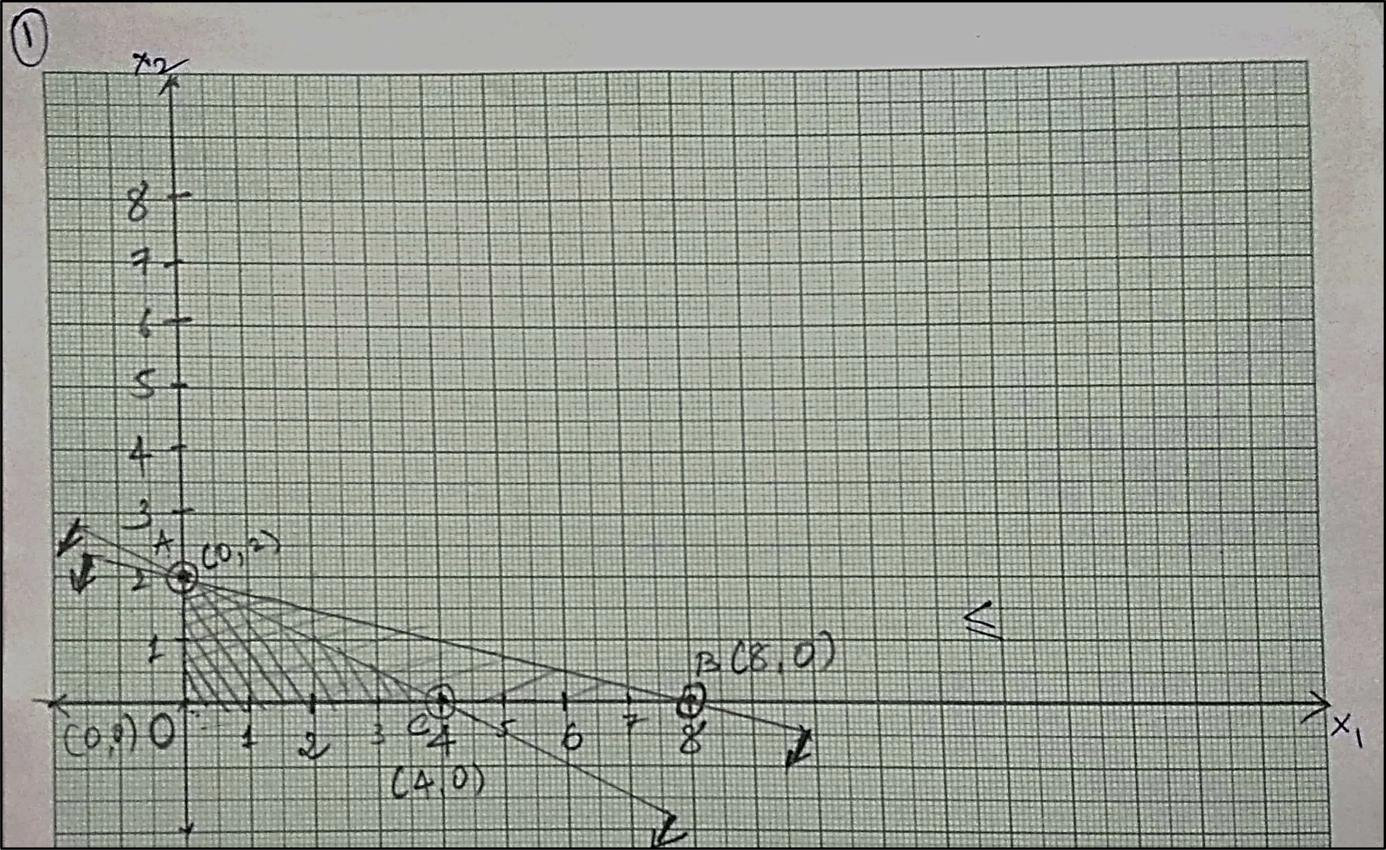
As inequalities of constraints in , selecting the region on and towards the origin of constraint lines.
For optimal solution, computing the value of objective function using extreme points of feasible region obtain from graph:
| Points | |
|---|---|
| (0,2) | |
| (0,0) | |
| (4,0) |
As objective is to maximize the profit, selecting maximum computed value of objective function, i.e.
Solution:
Numerical #2
Use graphical method to solve the following LPP
Solution #2
Solving the constraints by converting them into equation:
| Equation | 20x₁ + 30x₂ ≥ 900 | 40x₁ + 30x₂ ≥ 1200 | ||
|---|---|---|---|---|
| x₁ | 0 | 45 | 0 | 30 |
| x₂ | 30 | 0 | 40 | 0 |
Plotting the values in graph and using and we will be using Extreme corner point method:
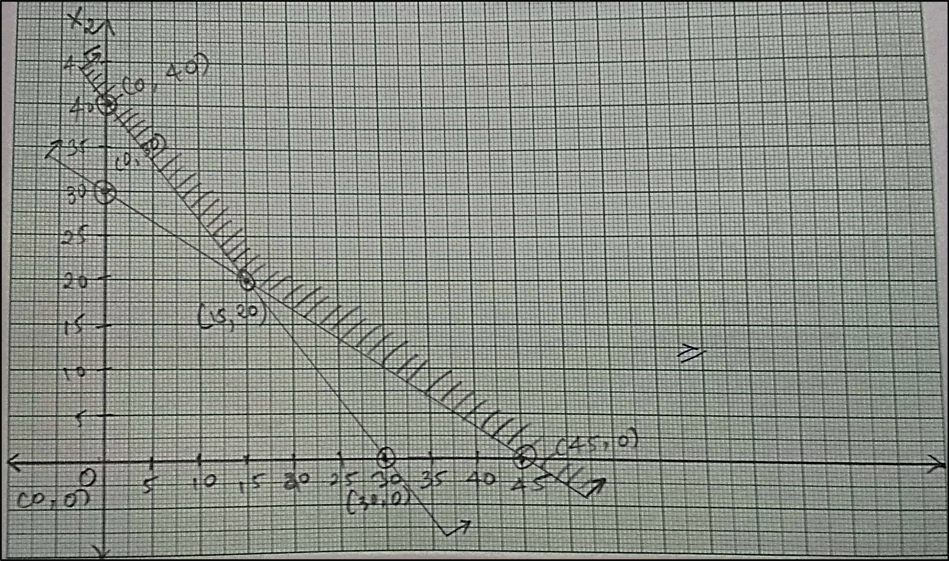
As inequalities of constraints in , selecting the region on and away of the constraint lines.
For optimal solution, computing the value of objective function using extreme points of feasible region obtain from graph:
| Points | |
|---|---|
| (0,40) | |
| (15,20) | |
| (45,0) |
As objective is to minimize the cost, selecting minimum computed value of objective function, i.e.
Solution:
Suggested Notes:
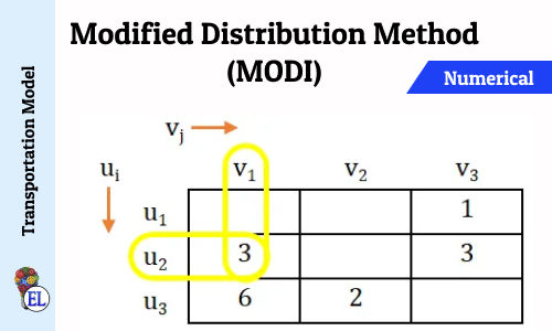
Modified Distribution Method (MODI) | Transportation Problem | Transportation Model
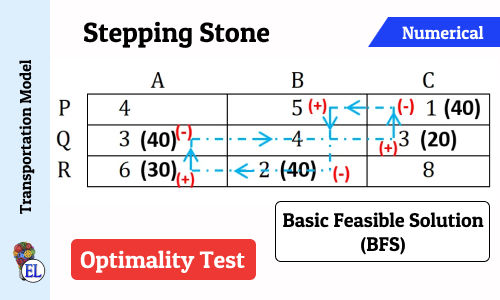
Stepping Stone | Transportation Problem | Transportation Model
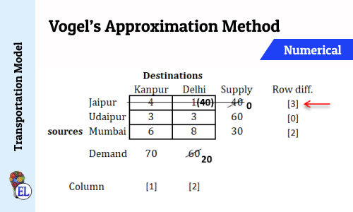
Vogel’s Approximation Method (VAM) | Method to Solve Transportation Problem | Transportation Model
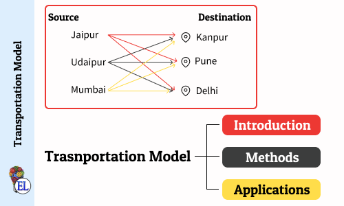
Transportation Model - Introduction
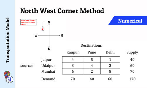
North West Corner Method | Method to Solve Transportation Problem | Transportation Model
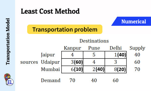
Least Cost Method | Method to Solve Transportation Problem | Transportation Model
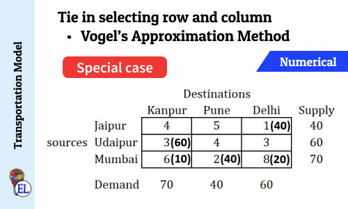
Tie in selecting row and column (Vogel's Approximation Method - VAM) | Numerical | Solving Transportation Problem | Transportation Model
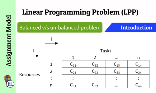
Assignment Model | Linear Programming Problem (LPP) | Introduction
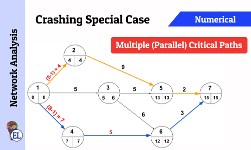
Crashing Special Case - Multiple (Parallel) Critical Paths
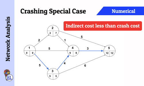
Crashing Special Case - Indirect cost less than Crash Cost
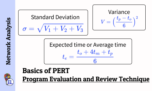
Basics of Program Evaluation and Review Technique (PERT)
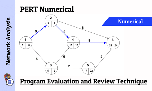
Numerical on PERT (Program Evaluation and Review Technique)

Network Analysis - Dealing with Network Construction Basics
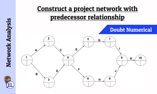
Construct a project network with predecessor relationship | Operation Research | Numerical
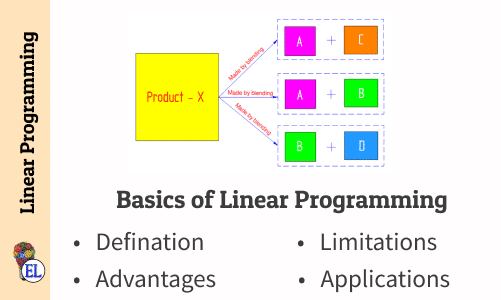
Basics of Linear Programming
Linear Programming Problem (LPP) Formulation with Numericals
Suggested Notes:
Modified Distribution Method (MODI) | Transportation Problem | Transportation Model
Stepping Stone | Transportation Problem | Transportation Model
Vogel’s Approximation Method (VAM) | Method to Solve Transportation Problem | Transportation Model
Transportation Model - Introduction
North West Corner Method | Method to Solve Transportation Problem | Transportation Model
Least Cost Method | Method to Solve Transportation Problem | Transportation Model
Tie in selecting row and column (Vogel's Approximation Method - VAM) | Numerical | Solving Transportation Problem | Transportation Model
Assignment Model | Linear Programming Problem (LPP) | Introduction
Crashing Special Case - Multiple (Parallel) Critical Paths
Crashing Special Case - Indirect cost less than Crash Cost
Basics of Program Evaluation and Review Technique (PERT)
Numerical on PERT (Program Evaluation and Review Technique)
Network Analysis - Dealing with Network Construction Basics
Construct a project network with predecessor relationship | Operation Research | Numerical
Basics of Linear Programming
Linear Programming Problem (LPP) Formulation with Numericals
Comments:
All comments that you add will await moderation. We'll publish all comments that are topic related, and adhere to our Code of Conduct.
Want to tell us something privately? Contact Us
Post comment